FarmTest: Factor Adjusted Robust Multiple Testing =================================================
Goal of the package
This R package conducts multiple hypothesis testing of mean effects. It implements a robust procedure to estimate distribution parameters and accounts for strong dependence among coordinates via an approximate factor model. This method is particularly suitable for high-dimensional data when there are thousands of variables but only a small number of observations available. Moreover, the method is tailored to cases when the underlying distribution deviates from Gaussianity, which is commonly assumed in the literature. See the papers on this method, (Fan et al. 2017) and (Zhou et al. 2017), for detailed description of methods and further references.
The observed data X is assumed to follow a factor model X = mu + Bf + u, where f are the underlying factors, B are the factors loadings, u are the errors, and mu is the mean effect to be tested. We assume the data is of dimension p and the sample size is n, leading to p hypothesis tests.
Installation
You can install FarmTest from github with:
install.packages("devtools")
devtools::install_github("kbose28/FarmTest")
library(FarmTest)
Getting help
Help on the functions can be accessed by typing “?”, followed by function name at the R command prompt.
Issues
-
Error: “…could not find build tools necessary to build FarmTest”: Since
FarmTestrelies onC++code, command line tools need to be installed to compile the code. For Windows you need Rtools, for Mac OS X you need to install Command Line Tools for XCode. See (https://support.rstudio.com/hc/en-us/articles/200486498-Package-Development-Prerequisites). -
Error: “library not found for -lgfortran/-lquadmath”: It means your gfortran binaries are out of date. This is a common environment specific issue.
-
In R 3.0.0 - R 3.3.0: Upgrading to R 3.4 is strongly recommended. Then go to the next step. Alternatively, you can try the instructions here: http://thecoatlessprofessor.com/programming/rcpp-rcpparmadillo-and-os-x-mavericks-lgfortran-and-lquadmath-error/.
-
For >= R 3.4.* : download the installer from the here: https://gcc.gnu.org/wiki/GFortranBinaries#MacOS. Now simply run the installer. (If installer is not available for your version of OS, use the latest one.)
-
-
Error: “… .rdb’: No such file or directory” Try devtools::install_github(“kbose28/FarmTest”, dependencies=TRUE)
-
Error in RStudio even after installing XCode: “Could not find tools necessary to build FarmTest”: This is a known bug in RStudio. Try options(buildtools.check=function(action) TRUE) in RStudio to prevent RStudio from validating build tools.
Functions
There are five functions available.
farm.test: The main function farm.test which carries out the entire hypothesis testing procedure. Has a print method.farm.FDR: Apply FDR control to a list of input p-values. This function rejects hypotheses based on a modified Benjamini- Hochberg procedure, where the proportion of true nulls is estimated using the method in (Storey 2015).farm.scree: Estimate the number of factors if it is unknown. The farm.scree function also generates two plots to illustrate how the number of latent factors is calculated. Has a print and plot method.farm.mean: Multivariate mean estimation with Huber’s loss.farm.cov: Multivariate covariance estimation with Huber’s loss.
Simple hypothesis testing example
Here we generate data from a factor model with 3 factors. We have 50 samples of 100 dimensional data. The first five means are set to 2, while the other ones are 0. We conduct a hypotheses test for these means.
library(FarmTest)
set.seed(100)
p = 100
n = 50
epsilon = matrix(rnorm( p*n, 0,1), nrow = n)
B = matrix(runif(p*3,-2,2), nrow=p)
fx = matrix(rnorm(3*n, 0,1), nrow = n)
mu = rep(0, p)
mu[1:5] = 2
X = rep(1,n)%*%t(mu)+fx%*%t(B)+ epsilon
output = farm.test(X, cv=FALSE)#robust, no cross-validation
output
#>
#>  One Sample Robust Test with Unknown Factors
#>
#> p = 100, n = 50, nfactors = 3
#> FDR to be controlled at: 0.05
#> alternative hypothesis: two.sided
#> hypotheses rejected:
#>  6
The robustness is controlled by the parameter of the Huber loss function. This can be chosen by cross-validation which takes a long time, but gives good results. Alternatively, we use the parameter tau * sd* * *rate where tau is a constant, rate is the optimal rate for the tuning parameter. See (Fan et al. 2017). sd is the standard deviation of the data at hand. The value of tau can be supplied by the user and takes a default value of 2.
##examples of other robustification options
output = farm.test(X, robust = FALSE, verbose=FALSE) #non-robust
output = farm.test(X, tau = 3, cv=FALSE, verbose=FALSE) #robust, no cross-validation, specified tau
#output = farm.test(X) #robust, cross-validation, longer running
Now we carry out a one-sided test, with the FDR to be controlled at 1%. Then we examine the output
output = farm.test(X, alpha = 0.01,alternative = "greater")
output
#>
#> One Sample Robust Test with Unknown Factors
#>
#> p = 100, n = 50, nfactors = 3
#> FDR to be controlled at: 0.01
#> alternative hypothesis: greater
#> hypotheses rejected:
#> 5
names(output)
#> [1] "means" "stderr" "loadings" "nfactors" "pvalue"
#> [6] "rejected" "alldata" "alternative" "H0" "robust"
#> [11] "n" "p" "alpha" "type" "significant"
print(output$rejected)
#> index pvalue pvalue adjusted
#> [1,] 3 5.512356e-74 2.867494e-72
#> [2,] 1 1.297040e-59 3.373561e-58
#> [3,] 5 1.074999e-45 1.864027e-44
#> [4,] 4 1.556500e-33 2.024205e-32
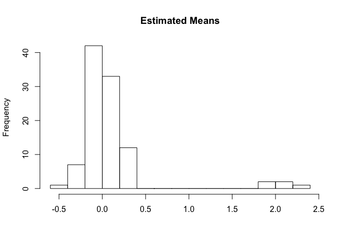
#> [5,] 2 1.798489e-10 1.871126e-09
hist(output$means, 10, main = "Estimated Means", xlab = "")
A two-sample test is done as follows:
n2 = 25
epsilon = matrix(rnorm( p*n2, 0,1), nrow = n2)
B = matrix(rnorm(p*3,0,1), nrow=p)
fy = matrix(rnorm(3*n2, 0,1), nrow = n2)
Y = fy%*%t(B)+ epsilon
output = farm.test(X=X,Y=Y)
output
#>
#>  Two Sample Robust Test with Unknown Factors
#>
#> p = 100, nX = 50, nY = 25, X.nfactors = 3, Y.nfactors = 3
#> FDR to be controlled at: 0.05
#> alternative hypothesis: two.sided
#> hypotheses rejected:
#>  5
print(output$rejected)
#>      index       pvalue pvalue adjusted
#> [1,]     4 1.034103e-29    1.034103e-27
#> [2,]     5 1.276966e-27    6.384831e-26
#> [3,]     1 1.147628e-17    3.825428e-16
#> [4,]     3 1.822131e-10    4.555326e-09
#> [5,]     2 6.040175e-10    1.208035e-08
names(output$means)
#> [1] "X.mean" "Y.mean"
Other functions
The function farm.scree makes some informative plots. It is possible to specify the maximum number of factors to be considered and the maximum number of eigenvalues to be calculated in this function. We recommend min(n,p)/2 as a conservative threshold for the number of factors; this also prevents numerical inconsistencies like extremely small eigenvalues which can blow up the eigenvalue ratio test.
output = farm.scree(X, K.factors = 15, K.scree = 10, show.plot = TRUE)
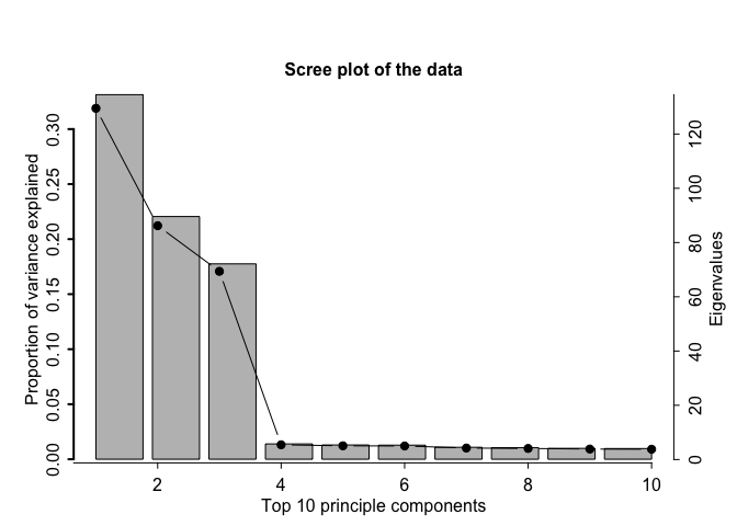
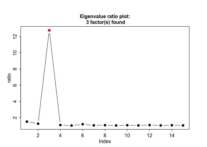
output
#> Summary of eigenvalue ratio test
#> Number of factors found: 3
#> Proportion of variation explained by the top 3 principal components: 72.94%
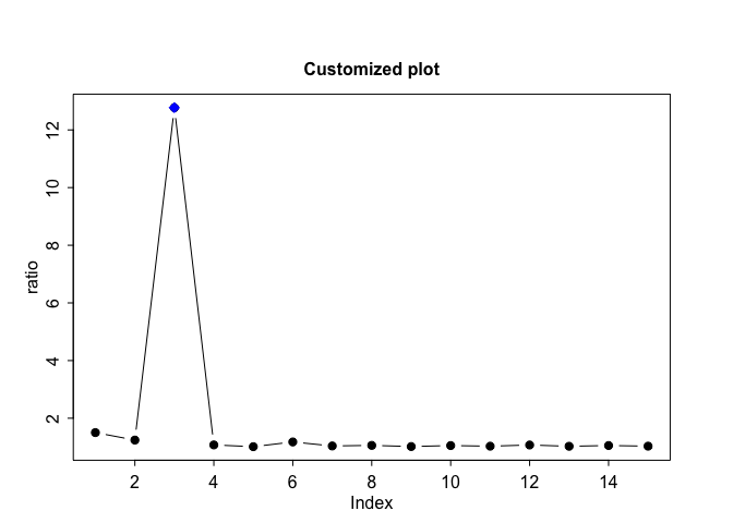
plot(output, scree.plot=FALSE, col="blue", main="Customized plot")
Let us generate data from a Gaussian distribution with mean 0. Suppose we perform a simple t.test in R and need to adjust the output p-values for multiple testing. The function farm.FDR lets us carry out multiple comparison adjustment and outputs rejected hypotheses. We see that there are no rejections, as expected from a zero-mean Gaussian distribution.
set.seed(100)
Y = matrix(rnorm(1000, 0, 1),10)
pval = apply(Y, 1, function(x) t.test(x)$p.value)
output = farm.FDR(pval)
output$rejected
#> [1] "no hypotheses rejected"
Finally let us calculate the mean and variance of our dataset.
muhat = farm.mean(X)
covhat = farm.cov(X)
Notes
-
If some of the underlying factors are known but it is suspected that there are more confounding factors that are unobserved: Suppose we have data X=mu + Bf + Cg + u, where f is observed and g is unobserved. In the first step, the user passes the data {X, f} into the main function. From the output, let us construct the residuals: Xres = X - Bf. Now pass Xres into the main function, without any factors. The output in this step is the final answer to the testing problem.
-
Number of rows and columns of the data matrix must be at least 4 in order to be able to calculate latent factors.
-
The farm.FDR function uses code from the
pi0estfunction in theqvaluepackage (Storey 2015) to estimate the number of true null hypotheses, and inherits all the options frompi0est. -
See individual function documentation for detailed description of methods and their references.
Fan, J., Y. Ke, Q. Sun, and W.-X. Zhou. 2017. “FARM-Test: Factor-Adjusted Robust Multiple Testing with False Discovery Control.” https://arxiv.org/abs/1711.05386.
Storey, J.D. 2015. “Qvalue: Q-Value Estimation for False Discovery Rate Control.” R Package Version 2.8.0. http://github.com/jdstorey/qvalue.
Zhou, W.-X., K. Bose, J. Fan, and H. Liu. 2017. “A New Perspective on Robust M-Estimation: Finite Sample Theory and Applications to Dependence-Adjusted Multiple Testing.” Annals of Statistics, to Appear. https://arxiv.org/abs/1711.05381.